2nd Derivative Test

After returning two old quizzes and giving today's quiz on concavity, I worked two example problems. The first illustrated the use of the 2nd derivative test. It's quite straightforward, but what students sometimes forget is that the 2nd derivative test is used to find relative extrema. Previously, we have used the 1st derivative test; now we have a second method for finding relative minimums and maximums.

The second example for today emphasizes the relationship between the 1st derivative, the 2nd derivative and the graphs of functions. This will be our focus of study for much of the next week.

Tomorrow's quiz will be a review quiz - it will cover some topic that a previous quiz was over.

Notes from today are attached below.

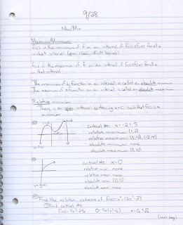
Minimums and Maximums

Today we learned about maximums and minimums. Important points:

-The absolute maximum/ minimum could be the end points of the interval, but the relative minimum/maximum could not (absolute: closed interval, relative: open interval).

-When finding the intervals where a function is increasing/decreasing, make sure the number line is drawn as shown in the notes.

-The relative minimum/maximum can be found when you draw the arrows on the number line, so you can see where the graph would be at its highest and lowest points.

Critical Numbers and Increasing/Decreasing Intervals

We didn't get to maximum/minimum or relative maximum/minimum today; that'll be tomorrow.

Basically, a critical number is a defined point (c,f(c)) on f(x) where f'(c) is zero or f'(c) is undefined. AKA when a function goes from increasing to decreasing or vice versa.

An interval [a,b] is increasing if f'(x)>0 for all x in (a,b)
An interval [a,b] is decreasing if f'(x)<0 for all x in (a,b)

The critical number can be used to find the increasing and decreasing intervals of a function. Make a number line, mark all critical numbers, and plug one number from each section created into the derivative equation to determine increasing and decreasing intervals.

September 23 - Proof by contradiction and MVT

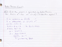
As we learned yesterday, the Mean Value Theorem is essentially Rolle's Theorem generalized so the two points (a,b) do not have to output the same y-value. We did not have a quiz today, but we will on Monday involving the Mean Value Theorem in an "interesting" way. Last night's homework applied the MVT to finding the c value guaranteed by the theorem and to a proof (p.176 #79). This proof, however, involved more algebra than it did calculus.

In class yesterday, we were first introduced to Proof by Contradiction with an example. This method of proof requires that in order to prove a statement, you must show that everything besides that statement is not possible. The difficulty in these type proofs is determining how to approach it and making a supposition to disprove.

Today in class we worked another example of a Proof by Contradiction. The homework tonight includes 3 such proofs.

Notes from today are below.

September 22 - The Mean Value Theorem

The Mean Value Theorem is a generalization of Rolle's Theorem (covered yesterday). In Rolle's Theorem, the function had to have the same y coordinate at the endpoints of the interval. The Mean Value Theorem addresses a function over any interval and essentially says that the average (mean) rate of change of a function over some interval will equal the instantaneous rate of change of the function somewhere in the interval.

You will see some generic problems finding the c value guaranteed by the MVT. We will also work some proofs using the MVT. One mathematical method of proof that you will need to use is called "Proof by Contradiction" and I worked an example of this in class today.

Notes from today are below.

September 21 - Rolle's Theorem

We begin Chapter 3 with Rolle's Theorem. This is the first of several theorems that we will talk about that describe the behavior of what I have previously called "nice" functions. That is, we are better defining "nice."

Rolle's Theorem is actually a silly sort of theorem. Generalized, it becomes a more powerful and important statement about functions; alas, poor Rolle didn't generalize and so didn't get the greater glory that could have been his. (Lagrange would eventually prove the Mean Value Theorem - we will cover this tomorrow.)

Another new concept that we covered today is the idea of differentiability. We have previously talked about when a function is continuous. Now you should be able to describe when a function is differentiable. Intuitively, if a function has a "sharp point" (absolute value, x^(2/3)), then it is not differentiable at that sharp point. Additionally, if a function is not continuous at some x = c, then it is also not differentiable at x = c.

Notes from today are below.

September 8 - The Chain Rule

The Chain Rule is the rule for the composition of functions - that is one function is "inside" another, ie f(x) = a(b(x)). The Chain Rule is an all encompassing rule - you have already been using it though it hasn't been apparent.

The thought process for using the Chain Rule is to think

"The derivative of f(x) will be the derivative of the outside function times the derivative of the inside function."

The trick is that when you differentiate the "outside function," you don't change the function on the inside. That probably doesn't make sense to read, but ultimately, with practice, I think you will come to understand.

Notes from today are shown below and include several worked examples.

September 7 - Product and Quotient Rules continued

As far as the derivative rules go, there wasn't anything new.

A consequence of now having the quotient rule is that we can now differentiate all six trig functions. You are now responsible for each of those derivatives:

d(sin x)/dx = cos x
d(tan x)/dx = (sec x)^2
d(sec x)/dx = sec x tan x

d(cos x)/dx = -sin x
d(cot x)/dx = -(csc x)^2
d(csc x)/dx = -csc x cot x

There is a nice pattern to the derivatives that should make it a little easier to memorize them. Better to have them learned sooner than later.

September 2 - The Product and Quotient Rules

Today we introduced two more rules for finding derivatives of functions. Previously we have seen (seemingly silly) rules for finding the derivatives of sums or differences. The derivative of a function that was defined as a sum (f(x) = a(x) + b(x)) is simply the sum of the derivatives (f'(x) = a'(x) + b'(x)). Similarly for differences.

It turns out the patterns for products and quotients are a little more complicated. I am opting not to show you where the formulas come from, but you are certainly encouraged to look up the proofs in your text.

Notes from class today include the Product Rule, the Quotient Rule and several worked examples.